Supplementary Figure 7. Comparison of single population genetic statistics and deep learning models for differentiating between positive selection and neutral evolution. To evaluate each method, we simulated approximately 2.8 million synthetic tumours across different mean sequencing depths (50, 75, 100, 125, 150, 200, 250x) and sequencing overdispersion parameters (0, 0.001, 0.003, 0.01, 0.03). Sequencing overdispersion refers to the rho parameter of the beta distribution in a beta-binomial sequencing noise model. An overdispersion parameter of 0.01 is a rough upper limit for empirical data (based on sequencing noise model outlined in Williams et al. 2018). The mutation rate was set to 100 mutations per cell division per genome. (a) ROC curves for each sequencing depth and dispersion combination where columns indicate sequencing dispersion (see top text) and rows indicate sequencing depth (see right text). For each non-TumE statistic, the optimal threshold/cutoff value for specifying positive selection was determined by maximizing the sensitivity and specificity in a cutpoint analysis using cutpointr. (b) The median AUROC across all sequencing depth and overdispersion parameters for each method. TumE - Mean refers to calling positive selection if the mean of the approximate posterior density was greater than 0.5 for P(Selection). TumE - L89% refers to calling positive selection if the lower bound of an 89% equal-tailed interval was greater than 0.5 for P(Selection). (c) The precision and recall for calling positive selection using different approximate posterior cutoffs (mean or lower bound of 89% equal-tailed interval) at increasing sequencing depth.

Supplementary Figure 8. Predicting the number of subclones (0, 1, 2) in 2.8 million synthetic tumours. To evaluate each method, we simulated approximately 2.8 million synthetic tumours across different mean sequencing depths (50, 75, 100, 125, 150, 200, 250x) and sequencing overdispersion parameters (0, 0.001, 0.003, 0.01, 0.03). We computed precision and recall across for predicting 0, 1, or 2 subclones. (a) Precision and (b) recall for prediction of 0 subclones. (c) Precision and (d) recall for prediction of 1 subclone. (e) Precision and (f) recall for prediction of 2 subclones. MOBSTER refers to the population genetics mixture model developed by Caravagna et al 2020. For MOBSTER, we assigned the number of subclones as outlined in the original paper. We assigned 1 subclone if there was a clonal cluster (C1), a neutral tail, and a subclonal cluster (C2), or if there was a clonal cluster (C1), and two subclonal clusters (C2 and C3). We assigned 2 subclones if there was a clonal cluster (C1), a tail, and two subclonal clusters (C2 and C3). All samples with only a clonal cluster (C1) or a clonal cluster and a neutral tail were assigned 0 subclones. .

Supplementary Figure 9. Correlation between true subclone frequency and predicted subclone frequency using synthetic supervised learning (TumE) and a population genetics informed mixture model (MOBSTER; Caravagna et al. 2020). We simulated approximately 1 million synthetic tumours with one subclone between 9 - 41% VAF across a range of sequencing depths (50 – 250x) and overdispersion parameters rho (0 – 0.03). To enable a reasonable comparison against the mixture model approach we only evaluated correlations where the predicted number of subclones for a given method matched the true number of subclones. We find strong agreement between both methods at higher sequencing depths. However, we note that the mixture model approach took approximately 24 hours using 500 cores to analyze >1 million synthetic tumours. Conversely, the trained neural network took a similar amount of time while using only one core. .

Supplementary Figure 10. Error in predicting frequency of 2 detectable subclones with synthetic supervised learning (TumE). We simulated approximately 500,000 synthetic tumours with 2 subclones located between 9 – 41% VAF. Our simulations covered sequencing depths from (50 – 250x) and sequencing overdispersion parameters (0 - 0.03). Each panel shows the predicted error (true frequency - predicted frequency) for the highest frequency subclone (Subclone 1) and lowest frequency subclone (Subclone 2) in each of the 500,000 VAF distributions/synthetic tumours. The mean percentage error (MPE) for predicting Subclone 1 and 2 is provided at each sequencing depth and overdispersion combination. The color of each point is the L1 loss or mean absolute error for each sample. .

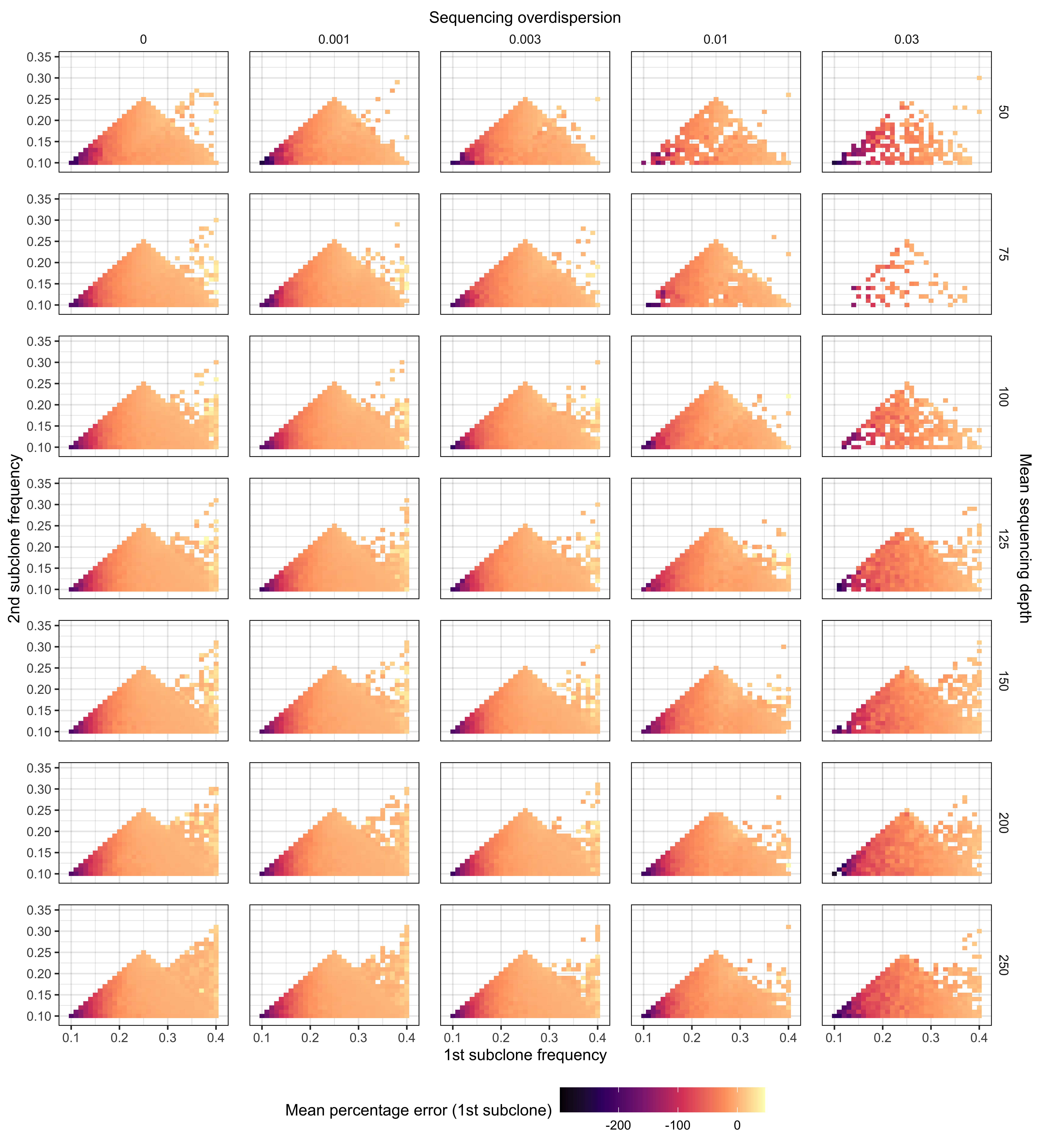
Supplementary Figure 11. Relationship between frequencies of subclones in the 2 subclone setting and the mean percentage error for the highest frequency subclone (1st subclone). We simulated approximately 500,000 synthetic tumours with 2 subclones located between 9 – 41% VAF. Our simulations covered sequencing depths from (50 – 250x) and sequencing overdispersion parameters (0 - 0.03). For frequency intervals/bins of 0.1 VAF, the mean percentage error was computed for predicting the 1st subclone frequency.

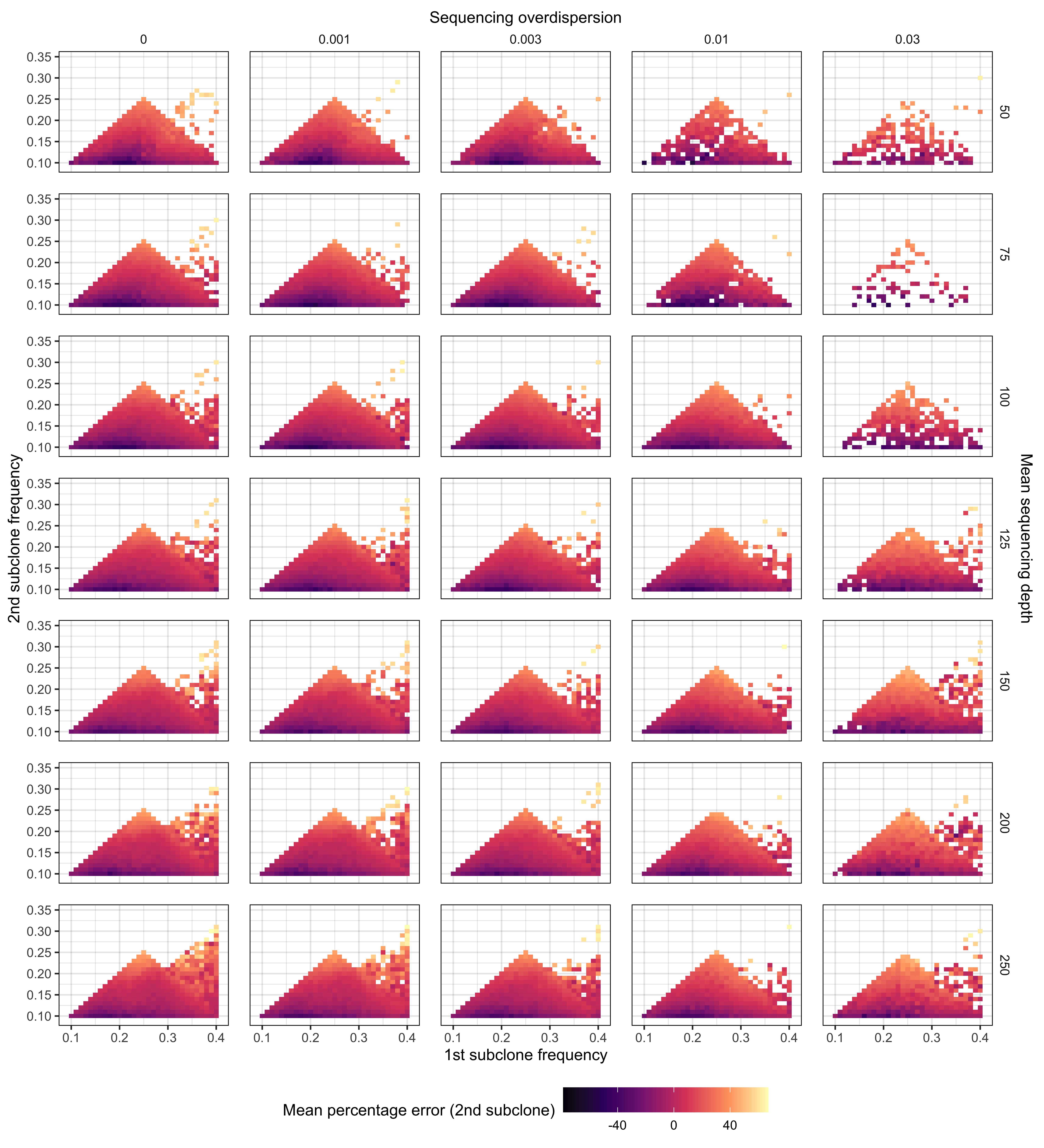
Supplementary Figure 12. Relationship between frequencies of subclones in the 2 subclone setting and the mean percentage error for the lowest frequency subclone (2nd subclone). We simulated approximately 500,000 synthetic tumours with 2 subclones located between 9 – 41% VAF. Our simulations covered sequencing depths from (50 – 250x) and sequencing overdispersion parameters (0 - 0.03). For frequency intervals/bins of 0.1 VAF, the mean percentage error was computed for predicting the 2nd subclone frequency.